Self Diagnosis of Periodic Limb Movement Disorder Using Python & OpenCV

Intro

So for years I’ve always felt excessive daytime sleepiness and fatigue. Once I finally got a job after school I now had health insurance and money to start looking into the issue. I visited a sleep doctor and was told “without even doing a sleep study I can already tell there’s a 75% chance you have sleep apnea”. Long story short after a $1000 sleep study the end result was almost zero sleep apnea and no issues identified at all. Basically I was told I’m fine.

I wasn’t happy with that answer since I knew there was something up. I decided to record some video to look into what I might be doing at night.

Hardware

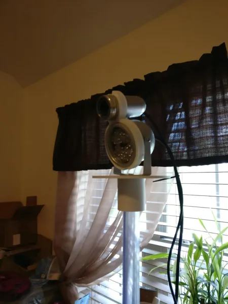
I took a $10 webcam and removed the IR filter from it. Any webcam will do but the $10 one worked great for this. I also got a $10 IR light from Amazon (48 led night vision illuminator). I set this up a few feet past the foot of my bed. I used some clear PVC pipe I had on hand to setup a 3d printed mount so that the camera was about 5 feet higher than where I slept.

Data Analysis

Alright so after this I ended up with around 1.2 GB of video, but what do you do from there? I tried watching a little bit and scanning manually skipping around but it was tough to find anything interesting. So I decided to learn some Python and OpenCV to analyze what was happening.

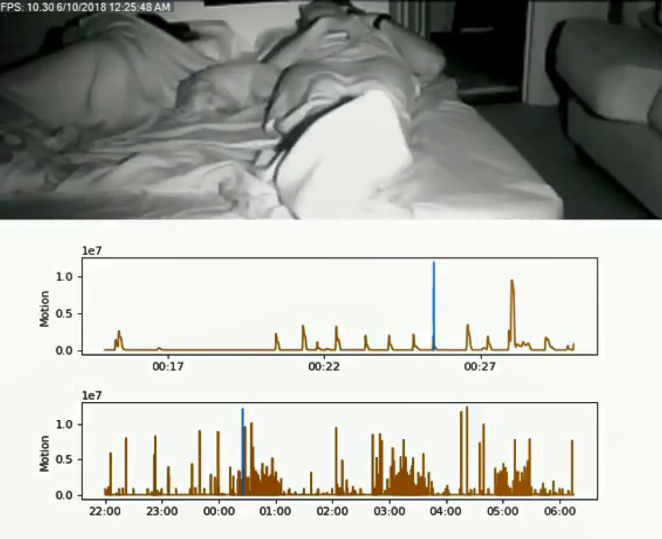
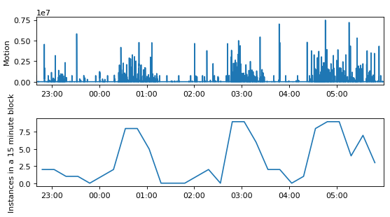
The OpenCV part was pretty straightforward. I used a background subtract function which is normally used for motion tracking/highlighting. Rather than using the mask to highlight parts of the video, I used the mask to calculate how much activity was happening in a given frame. Simply summing up the mask array gives you a value that describes frame by frame activity. A high value means a lot of pixels have changed from one frame to the next. This condenses the data of every frame down to a single 2-byte or so value and we calculate an average every second to further reduce the data. So that condenses the data we need to interpret from from 1.2GB of information down to ~100kB. That’s a factor of 10,000 in reduction and makes our job a little easier. We can use that to generate the simple plot shown below.

So this plot very generally shows us where there is activity throughout the night. Again, I found this kind of hard to interpret but it started pointing me in the right direction. It definitely looks like something’s going on here, but what? The next step was to make a compilation video so I could see exactly what this activity was. Another quick observation at this point was that the activity seems to happen in episodes throughout the night that last about an hour. At this point it made sense that the periods of low activity are probably deep REM sleep and that something is happening outside of that. The first compilation video I made is the youtube link below.

Based on the compilation video I could now see I have a lot of foot and leg movements in hour long episodes and there are a few of those episodes a night. At first I was searching about restless leg syndrome but that is something that affects people while awake. But I started to find mentions of “periodic limb movement disorder” alongside the RLS. This disorder is specifically involuntary during sleep and you will have hour long episodes where you have movements every minute or two with multiple episodes a night. That was the “AHA” moment. It felt good to finally have an explanation for my fatigue. The $1000 sleep study I had specifically had a section on PLMD and said I scored 0.0 – absolutely no movements. I asked the PA how they quantify that and apparently it’s based on leg electrodes – I don’t remember them putting leg electrodes on me and when I asked to see the data I never did get a clear answer on if it exists.

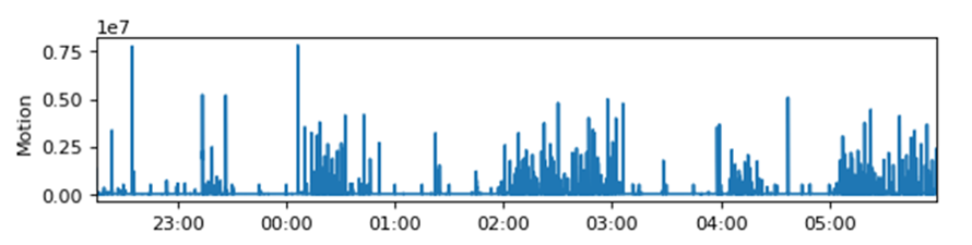
Another data reduction we can do on the activity plot is to count up the number of kicks/events in a given time interval and plot that (shown below). You could use this to determine PLM index since this is the # of distinct kicks/movements throughout the night.

Conclusion

So with a day’s work I was able to take an intimidating mountain of data and turn it into a simple plot of 32 data points that also has medical diagnostic relevance (PLMD index). While it’s kind of nice having disorder identified, I haven’t really found a fix yet. PLMD isn’t really the root cause, just a description of symptoms.

flowchart LR
    id1["8 Hours of Webcam feed
    1.2 GB"]
    id2["Motion Tracking Data
    100 kB"]
    id3["Kick/Event Data
    1 kB"]
    id1 -->|"OpenCV
    10,000x reduction"| id2
    id2 -->|"Python
    100x reduction"| id3

Code

Here’s the code that generated the plots above.

import os
import cv2
import winsound
import numpy as np
import matplotlib.pyplot as plt
import datetime as dt
import matplotlib.dates as mdates

#set the proper start time for your video files. Also set the directory containing the video files
videoStartDate = dt.datetime(year = 2018, month = 10, day = 17, hour=22, minute=52, second=39)
vidDirectory = r"C:\Users\Glow-PC\Documents\OpenCV Sleep\20181017"
#get a list of all files and then trim that list down to mp4 files. the default naming scheme from iSpy keeps things in chronological order
fileList = os.listdir(vidDirectory)
videoList = []
for f in fileList:
    if f.endswith('.mp4'):  
        videoList += [f]

#these 4 numbers define the region of interest for my legs. Make sure it captures from the knees down to below the feet.
nickMaskX1 = 50
nickMaskX2 = 250
nickMaskY1 = 200
nickMaskY2 = 420

#choose a random video file (15th in this case) so that we can fine tune the region of interest above. hit escape to leave vid
vid = videoList[15]   
vidCap = cv2.VideoCapture(vid)  


while(True):
    ret, frame = vidCap.read()
    if not ret:
        break

    cv2.rectangle(frame,(nickMaskX1,nickMaskY1),(nickMaskX2,nickMaskY2),(0,0,255),15)
    cv2.imshow('frame1',frame)
    k = cv2.waitKey(1) & 0xFF
    if k == 27:
        break

vidCap.release()
cv2.destroyAllWindows()

#now that we have defined the ROI we step through the video files in order and extract "activity data"
#calculate the average "activity" in a given second and then save the data point.
#we use the background subtract feature in openCV that can be used to highlight motion in a video feed
#the value we care about is just the sum of the mask in the ROI. high value = lots of pixels have changed
#every video file (in my case 15 min video files) gets its own output txt file that is simply a 1D list of activity values for every second
for vid in videoList:
    
    listString = list(vid)
    listString = listString[:-4]
    listString = listString + list("IndivAct") + list(".txt")
    newExtension = ''.join(listString)
    activityFile = open(newExtension,"w+")
    
    cap = cv2.VideoCapture(vid)
    fgbg = cv2.createBackgroundSubtractorMOG2()
    
    prevMilliTimer = 0
    nickRunningSum = 0 
    meanIndex = 0

    while(True):
        ret, frame = cap.read()
        if not ret:
            break

        fgmask = fgbg.apply(frame)

    #check ms of video, collect data for 1s and once you roll over into the next second save the data and reset variables    
        currentMilliTimer = cap.get(cv2.CAP_PROP_POS_MSEC) % 1000

        if currentMilliTimer < prevMilliTimer: #if true then we rolled into the next second
            activityFile.write(str(nickRunningSum / meanIndex)) #my activity
            activityFile.write("\r")
            nickRunningSum = 0
            meanIndex = 0

        nickRunningSum += np.sum(fgmask[nickMaskY1:nickMaskY2,nickMaskX1:nickMaskX2]) #keep a running sum of the nick activity that we'll average every 1s
        meanIndex += 1 #this var will divide to make mean
        prevMilliTimer = currentMilliTimer
        
    print(vid)
    cap.release()
    cv2.destroyAllWindows()
        
    activityFile.close()

#this is just so I get a system beep once completed
frequency = 1000  # Set Frequency To 2500 Hertz
duration = 250  # Set Duration To 1000 ms == 1 second
winsound.Beep(frequency, duration)

#make a list of the txt activity files that we generated above, then import it into 1 array
fileList = os.listdir(vidDirectory)
dataFileList = []
for f in fileList:
    if f.endswith('IndivAct.txt'):
        dataFileList += [f]
        
with open(dataFileList[0], 'rU') as dataFileObj:
    dataList = [1] #put a dummy value here and drop it later
    for line in dataFileObj:
        lineArray = int(float(line))
        dataList = np.append(dataList,lineArray)
    dataList = dataList[1:]
for x in range(1,len(dataFileList)):
    with open(dataFileList[x], 'rU') as dataFileObj:
        for line in dataFileObj:
            lineArray = int(float(line))
            dataList = np.append(dataList,lineArray)
#our activity data files were 1D arrays of our Y-value, here we generate our 1D array of X-values (time)            
timeArray = [videoStartDate + dt.timedelta(seconds = i) for i in range(len(dataList))]
quarterHourTimeArray = [videoStartDate + dt.timedelta(minutes = 7.5+15*i) for i in range(round(len(dataList)/900))]

#threshold/binarize the data. 1E6 worked really well for all of my work.
#any time that is >threshold gets accumulated in an array
eventData = []
threshold = 1E6
for x in range(0,len(dataList)):
    if dataList[x] > threshold:
        eventData = np.append(eventData,timeArray[x])

#now we have a long list of time values, but multiple sequential time values are really just one kick or movement
#so lets condense that array down to an array of "events"
#we're looking for rising edges and falling edges of our digital/binarized data
#the >2 part below basically says if two events are within 2 seconds of each other, ID them as 1 event
#in the end the eventList array is a 1D list of start and end times of the events we have identified
#example: eventData may contain a series [3,4,5,10,11,12] 
#which then gets ID's as two events and would have eventList=[3,5,10,12]

midEventFlag = False
eventList = []
for x in range(0,len(eventData)-1):
    if not midEventFlag:
        eventList = np.append(eventList,eventData[x])
        midEventFlag = not midEventFlag
    else:
        if (eventData[x + 1] - eventData[x]).total_seconds() > 2:
            eventList = np.append(eventList,eventData[x])
            midEventFlag = not midEventFlag
#now take our eventList and figure out 1) how long the event lasted and 2) what time was the event (the middle of the event)
eventTime = []
eventDuration = [] 
for x in range(0,len(eventList)-1,2):
    eventMidTime = eventList[x]+dt.timedelta(seconds = int((eventList[x+1]-eventList[x]).total_seconds()/2))
    eventTime = np.append(eventTime, eventMidTime)
    eventDuration = np.append(eventDuration, eventList[x+1]-eventList[x])

#now tally up the # of events we find in a 15 minute block
histoList = []
for x in range(0,len(quarterHourTimeArray)):
    histoList = np.append(histoList, len([element for element in eventTime if element>videoStartDate + dt.timedelta(minutes = 15*x) and element<videoStartDate + dt.timedelta(minutes = 15*(x+1))]))

    myFmt = mdates.DateFormatter('%H:%M')
fig = plt.figure(num=0, figsize=(8, 4), dpi=80, facecolor='w', edgecolor='k')
ax1 = fig.add_subplot(212)
ax2 = fig.add_subplot(211)

ax1.plot(quarterHourTimeArray,histoList)
ax1.set_ylabel('Instances in a 15 minute block')
ax1.xaxis.set_major_formatter(myFmt)
ax1.set_xlim([timeArray[0],timeArray[-1]])


ax2.plot(timeArray,dataList)
ax2.set_ylabel('Motion')
ax2.xaxis.set_major_formatter(myFmt)
ax2.set_xlim([timeArray[0],timeArray[-1]])

fig.subplots_adjust(wspace=0, hspace=0.5)

#the print below is the total # of kicks/events in the night
print(len(eventTime))

#this section is to generate a compilation video of events through the night with a corresponding activity plot
#this part is unnecessary most of the time but was important while initally understanding the data
#secondsIn and videoIndex pick a random video and a time within that video to make sure our plots are coming out right
myFmt = mdates.DateFormatter('%H:%M')
secondsIn=5400
videoIndex=6
lineTime= timeArray[0] + dt.timedelta(seconds = secondsIn)

fig = plt.figure(num=0, figsize=(8, 4), dpi=80, facecolor='w', edgecolor='k')
ax1 = fig.add_subplot(211)
ax2 = fig.add_subplot(212)

ax1.plot(timeArray[videoIndex*900:(videoIndex+1)*900],dataList[videoIndex*900:(videoIndex+1)*900])
ax1.plot([lineTime,lineTime],[0,1.2E7])
ax1.set_ylabel('Motion')
ax1.xaxis.set_major_formatter(myFmt)

ax2.plot(timeArray,dataList)
ax2.plot([lineTime,lineTime],[0,1.2E7])
ax2.set_ylabel('Motion')
ax2.xaxis.set_major_formatter(myFmt)

fig.subplots_adjust(wspace=0, hspace=0.5)

def refreshPlots(videoIndex, secondsIn):
    ax1.cla()
    ax2.cla()
    
    lineTime= videoStartDate + dt.timedelta(seconds = secondsIn)
    
    ax1.plot(timeArray[videoIndex*900:(videoIndex+1)*900],dataList[videoIndex*900:(videoIndex+1)*900])
    ax1.plot([lineTime,lineTime],[0,1.2E7])
    ax1.set_ylabel('Motion')
    ax1.xaxis.set_major_formatter(myFmt)

    ax2.plot(timeArray,dataList)
    ax2.plot([lineTime,lineTime],[0,1.2E7])
    ax2.set_ylabel('Motion')
    ax2.xaxis.set_major_formatter(myFmt)

#now we start a new video file and go through the same process as above but instead of outputting activity txt files
#we output any frame above the threshold to video and also stitch an activity plot below the video. ned result is a compilation
fullFrameHeight = 380+4*80
fullFrameWidth = 640
fourcc = cv2.VideoWriter_fourcc(*'XVID')
out = cv2.VideoWriter('nickCompWithPlot.avi',fourcc, 10.0, (fullFrameWidth,fullFrameHeight))
fullFrameArray = np.zeros((fullFrameHeight,fullFrameWidth,3),np.uint8)

for videoIndex in range(0,len(videoList)):
    vid = videoList[videoIndex]

    cap = cv2.VideoCapture(vid)
    fgbg = cv2.createBackgroundSubtractorMOG2()
    while(True):
        ret, frame = cap.read()
        if not ret:
            break

        fgmask = fgbg.apply(frame)

        if np.sum(fgmask[nickMaskY1:nickMaskY2,nickMaskX1:nickMaskX2]) > threshold:
            secondsIn = int(cap.get(cv2.CAP_PROP_POS_MSEC) / 1000) + videoIndex*900
            refreshPlots(videoIndex, secondsIn)
            fig.canvas.draw()
            figImgData = np.fromstring(fig.canvas.tostring_rgb(), dtype=np.uint8, sep='')
            figImgData = figImgData.reshape(fig.canvas.get_width_height()[::-1] + (3,))

            fullFrameArray[0:380,0:fullFrameWidth] = frame[0:380,0:fullFrameWidth]
            fullFrameArray[380:fullFrameHeight,0:fullFrameWidth] = figImgData
            out.write(fullFrameArray)

    cap.release()
    print(vid)

out.release()

frequency = 1000  # Set Frequency To 2500 Hertz
duration = 250  # Set Duration To 1000 ms == 1 second
winsound.Beep(frequency, duration)

Dog Tax

For anyone who made it this far, here’s a funny dog tax that I caught on accident during this data analysis…